Projective Geometry & Image Formation
We all have our own intuition of pictures, but how can we capture that intuition? Even the Greek philosophers had their own understanding of pictures with Platon’s allegory of the cave. A picture captures the world, but with lower fidelity. Intuitively, anyone who’s ever been to Firenze can attest the pictures don’t do the Duomo any justice. In this post we’ll examine what is actually lost by photograpy through the lens of geometry and projections. By the end we’ll uncover what the Renaissance artists discovered empirically about perspective and vanishing points.
Camera Obscura - The Pinhole Camera Model
unknown illustrator, Public domain, via Wikimedia Commons
The camera obscura is a predecessor to the modern camera, and in more ways than one might realise. Interestingly, the geometry of the camera obscure is the foundation of how modern cameras work, namely the pinhole camera model.
We imagine a closed box with only one infinitesimally small hole (pinhole) letting light from the outside in. This hole will be the origin of our coordinate system, and is often named the optical center. We’ll define $z$ as the camera axis aligned with this hole normal to the outer surface, and any point along this direction will be denoted as having “depth”. All rays of light entering the hole at an angle $\theta$ to axis $z$ will enter the box with an identical angle $\theta$. We’ll now define the distance from the opening to the back of the box by $f$. For simplicity’s sake, let’s assume that every ray entering the pinhole hits the back of the box and not the sides. We’ll denote points on the back of the box with coordinates $x$ and $y$. Intuitively, since every ray entering the box will hit the back plane, they’ll have the same z-coordinate $f$. For a ray originating from a point $p$ outside the box with coordinates $\bf{X} = (X, Y, Z)^T$, what will the coordinates on the back plane be?
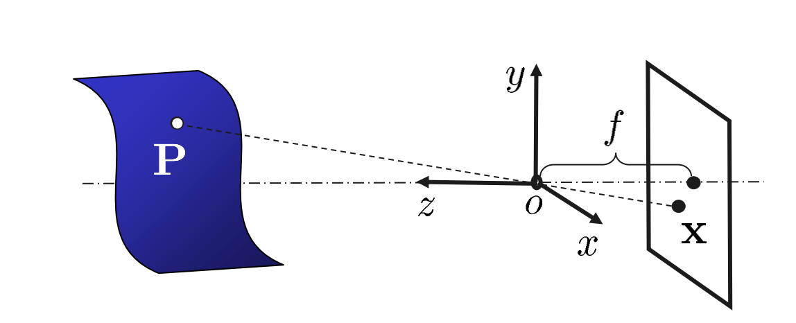
Copyright Martin Kleinsteuber
Self similar triangles give the relationship
\[\frac{x}{f} = -\frac{X}{Z}, \ \frac{y}{f} = -\frac{Y}{Z}, \ \frac{z}{f} = 1 \\\]We can see that the relationship between $x$ and $X$ and $y$ and $Y$ is linear by the same scaling factor $-f/Z$. In other words, the points on the back plane is just a scaled version of the origional point. We also note that the sign has changed, which means all points $p$ wil be upside down. But notice how $Z$ has no direct relation to $z$, but is linearly dependent on $x$ or $y$? This may seem uninteresting at first, but this fact houses many interesting insights. To illustrate this, imagine you’re inside the box viewing the point $(x,y)^T$. Now try to using the equations above, try to solve for $Z$ given $x,y,f$.
Impossible, right? So what does this tell us about the points or pictures we get of a point $p$ through the pinhole? It’s impossible to recover the depth $Z$ given the points on the back plane $(x,y)^T$. Consequently, since given $x, y, f$ the original point’s $X$ and $Y$ is defined to scale by $Z$, we can only recover the direction $X, Y$, and not actual scale. This may seem complicated at first, but what this means is that we are only able to know the direction a ray of light has come from, but not its depth $Z$. Expressing this relationship in vector form we get:
\[\begin{bmatrix} x \\ y \end{bmatrix} = -\frac{f}{Z}\begin{bmatrix} X \\ Y \end{bmatrix}\]for simplicity’s sake, we’ll drop the sign, which gives us the formula for ideal perspective projection
\[\begin{bmatrix} x \\ y\end{bmatrix} = \frac{f}{Z}\begin{bmatrix} X \\ Y \end{bmatrix}\]Notice that the right-hand side has three variables $(X, Y, Z)$, and the left-hand side has two variables $(x, y)$. In other words, we lose a dimension. We project $(X,Y,Z)^T \in \mathbb{R}^3$ to $(x, y)^T \in \mathbb{R}^2$.
\[\pi:\mathbb{R}^3 \rightarrow \mathbb{R}^2; \mathbb{X} \rightarrow \bf{x}\]We reduce the dimension of $(X, Y, Z)^T$ while keeping the direction of $(X, Y)$. Hence, we lose one-to-one uniqueness between the points we project and the projected point. Since we’re only able to recover the direction of $(X, Y, Z)^T$, any point $p$ along the same direction will project to the same point $\bf{x}$. How can we prove this, and what is the consequence?
Projective Geometry
As we’ve seen, images have a connection to scale invariance, that is “what stays the same when you scale (increase something’s size)”? This might seem obvious since images taken by a camera look the same on a phone as they do on a large TV screen. Images scale up and down without changing its contents, but why? Answering this question mathematically is less obvious, but by examining it we can discover some deep insigths and connections between images, projections, homogeneous coordinates and trigonometry.
The Projective Space
Proposition: Every point $p$ on a line through the pinhole/optical center $o$ projects to the same point $\bf{x}$. Consequently, for every point $x$ projected onto the back plane/image plane there exists exactly one line.
To prove this we have to introduce additional concepts and notation.
We’ll call two vectors equivalent to each other if there exists a $\lambda ≠ 0$ such that $x = \lambda y$. Then $x \sim y$ (equivalent). For example:
\[\begin{bmatrix} 1 \\ 0 \\ 0 \end{bmatrix} \sim \begin{bmatrix} 90 \\ 0 \\ 0 \end{bmatrix}\]In euclidean space $\mathbb{R}^n$ excluding the origin $x ≠ 0$ we can describe an equivalence class
\[[x] := \set{y\in \mathbb{R}^n \mid y \sim x}\]Which describes every line through the origin in $\mathbb{R}^n$. For example:
\[\left[{\begin{bmatrix} 2 \\ 2 \end{bmatrix}}\right] = \left[ \begin{bmatrix} 1 \\ 1\end{bmatrix}\right]\]Meaning the lines equvalent to $\begin{bmatrix} 2 \ 2 \end{bmatrix}$ are equal to the lines equivalent to $\begin{bmatrix} 1 \ 1 \end{bmatrix}$. With this notation we can define the projective space $\mathbb{P}^n$:
\[\mathbb{P}^n = \bf \set{\left[ x\right] \mid x \in \mathbb{R}^{n+1} \setminus \set{0} }\]Wow. That looks scary. What does this even mean? Reading it out we can see “The n-th dimensional projective space $\mathbb{P}^n$ is the set of all equivalent lines $[\bf x]$ in the $n +1$ dimensional Euclidean space $\mathbb{R}^{n+1}$ excluding the origin $\bf 0$.” It’s scary because it’s compact. We’ll need a bit more time to unpack every element of this definition, but I promise it will make sense in the end.
We’ll first examine the dimension of the projective space. Notice from the definition of $\mathbb{P}^n$ that it’s defined by the lines through the origin in one dimension more, i.e. $\mathbb{R}^{n+1}$. Since we’re used to three dimensions, we’ll first take a look at the projective space $\mathbb{P}^2$ since it’s expressed by the lines in $\mathbb{R}^3$.
Since lines are constrained to one dimension, the definition of the projective space $\mathbb{P}^2$ is simply the family of lines $L$ in $\mathbb{R}^3$ going through the origin $o$. But how can we express a line as a single point on the projective space? All lines in $\mathbb{R}^3$ can be expressed as the set of all vectors on the shell of a 3D ball $\mathbb{S}^2$ with any radius $r$, where a point $p$ and its opposite $p’$ represent the same point in the projective space, since $[p] \sim [p’], \ \lambda = -1$. We notice that the radius $r$ does not matter, neither does the sign of p. The only thing that distinguishes points in the projective space is direction.
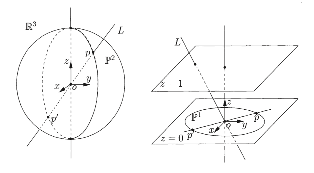
Yi Ma , Stefano Soatto , Jana Košecká , S. Shankar Sastryk /10.1007/978-0-387-21779-6
If instead of a ball we represent each point in the projective space $\mathbb{P}^2$ as the point where a line intersects a plane at $z = 1$ in $\mathbb{R}^3$, we get exactly one point / intersection per line, except for the line that lies on the plane $z = 0$. By using $z$ as a constraint, we get exactly the property we want for our projective space $\mathbb{P}^2$, namely uniqueness for every point $p$ in $\mathbb{P}^2$ where $z ≠ 0$. This works for any line with direction $(x, y, z)^T$ since we can always normalize such that $z=1$. But what about $z=0$? Imagine we have a vector $\bf x \in \mathbb{R}^3$ which we normalize such that:
\[\bf{x} =\begin{bmatrix} x/z \\ y/z \\ 1\end{bmatrix}\]As $z \rightarrow \infty $ $\bf x$ approaches direction
\[\bf{x} =\begin{bmatrix} x \\ y\\ 0\end{bmatrix}\]The the scale of $z$ becomes inconsequential in the limit, which means any point on $\mathbb{P}^2$ at infinity will converge to $ \left[\left[x, y, 0 \right] \right] $, which is on the plane $z=0$. This is by design, and is one of the genious attributes of the projective space. We can describe normal points in $\mathbb{P}^2$ as lying on the plane $z=1$ such that $[x, y, 1]^T$, and points at infinity are on the plane $z=0$ such that $[x,y,0]^T$. Incidentally, $[x,y,0]^T$ describes the circle $\mathbb{S}^1$ on the plane $z=0$, which is exacly the same as the projective space $\mathbb{P}^1$ by the same analogy as above. Therefore, $\mathbb{P}^2$ can be viewed as a 2D plane {$z=1$} with a circle $\mathbb{P}^1$ attached. The same argument can be used to define $\mathbb{P}^3$ etc.
This type of constraint which enforces the properties of points in a projective space, give rise to a new form of coordinates called homogeneous coordinates. We’ll examine homogeneous coordinates and figure out exactly what a point at infinity means, and how it applies to image formation.
Homogeneous Coordinates
Homogeneous coordinates stem from the fact that you can represent a point in one dimension in another, as long as we preserve the direction of the original vector. Two vectors
\[[X,Y, Z, 1] ^T, [XW, YW, ZW, W]^T \in \mathbb{R}^4\]Can be used to represent the same point $[X, Y, Z]$ in $\mathbb{R}^3$. The key is to realise that we haven’t actually changed the vector. This is exactly what we do when we constrain a point in $\mathbb{P}^2$ to the plane $z=1$. Going back to our camera, we can use $[x’, y’, z’]$ to represent a point $[x, y, 1]$ on the image plane $z = 1$, where $z$ is the distance from the optical center to the plane where points from outside intersect when going through the pinhole. Since our eyes work similar to the pinhole camera, we can actually use our own experience to link our understanding of projective geometry with how images are formed.
When we look around, we only capture what is in our image sphere. The objects we see are the lines / rays that go from the direction of the object to our eye. Any object in the same direction will be occluded by the origin of the ray we see. Objects further away look closer together, and objects near us look further apart, just like lines through a ball. The larger the radius, aka the distance, the further away objects are, and the closer they are on the sphere relative to the radius. How can we capture this intuition mathematically? And what about points at infinity?
Projective Geometry and Camera Projection
Using the definition of the projective space $\mathbb{P}^n$ we can realise that all points in $\mathbb{P}^n$ correspond to the homogeneous coordinates of the dimension $n+1$. The points corresponding to $\mathbb{P}^2$ are the vectors in $\mathbb{R^3}$ with at least one non-zero element
\[\mathbb{X} = [x_1, x_2, ..., x_{n+1}]^T, x_{n+1}≠0 \in \mathbb{R}^n\]We can normalize this vector by dividing it by $x_{n+1}$. With our newfound understanding we can realise that the pinhole camera coordinates $\bf x$ and $\lambda \bf{x}$ are equivalent ($\bf{x} \sim \lambda \bf{x}$) and represent the same point in the projective space $\mathbb{P}^2$, and therefore the same point on the image plane $z = f$.
Given the projection matrix $\Pi \in \mathbb{R}^{3x4}$, the camera model simply reduces to a transformation from a 3-dimensional projective space $\mathbb{P}^3$ to a 2-dimensional projective space $\mathbb{P}^2 $:
\[\Pi: \mathbb{P}^3 \rightarrow \mathbb{P}^2; \ \bf{X}_0 \rightarrow \bf{x}' \sim \Pi X_0\]From Pinhole Camera to Real Cameras
So far we’ve explored the ideal pinhole camera model, but real cameras are more complex. They have lenses, different focal lengths, and can be positioned and oriented anywhere in 3D space. To bridge this gap, we need to understand how the simple pinhole projection extends to a general camera model through the projection matrix $\Pi$.
The full projection matrix $\Pi$ can be decomposed into three main components:
\[\Pi = K\Pi_0 g = [KR, KT]\]Let’s break this down systematically to understand what each component represents.
The Canonical Projection Matrix $\Pi_0$
We start with the simplest case - the canonical projection matrix:
\[\Pi_0 = \begin{bmatrix} 1 & 0 & 0 & 0 \\ 0 & 1 & 0 & 0 \\ 0 & 0 & 1 & 0 \end{bmatrix}\]This $3 \times 4$ matrix performs the basic perspective projection we derived earlier. It takes a 3D point in homogeneous coordinates $\bf{X} = [X, Y, Z, 1]^T$ and projects it to:
\[\bf{x}' = \Pi_0 \bf{X} = \begin{bmatrix} X \\ Y \\ Z \end{bmatrix}\]After normalization by $Z$, we get the familiar pinhole camera equations: $x = X/Z$, $y = Y/Z$. This is exactly what we derived from similar triangles in the camera obscura.
Camera Pose: Rotation $R$ and Translation $T$
Real cameras aren’t always positioned at the origin looking down the $z$-axis. The matrix $g$ (often written as $\left[R\mid T\right]$) accounts for the camera’s position and orientation in the world:
- $R$: A $3 \times 3$ rotation matrix that describes how the camera is oriented relative to the world coordinate system
- $T$: A $3 \times 1$ translation vector that describes where the camera is located in world coordinates
The combined transformation is:
\[g = \begin{bmatrix} R & T \\ 0^T & 1 \end{bmatrix} \in \mathbb{R}^{4 \times 4}\]This transforms world coordinates to camera coordinates before projection. Think of it as accounting for where you’ve placed your camera in the world and which direction it’s pointing.
Intrinsic Camera Parameters: Matrix $K$
The matrix $K$ encodes the camera’s internal characteristics, namely things that depend on the camera itself, not where it’s placed:
\[K = \begin{bmatrix} f_x & s & c_x \\ 0 & f_y & c_y \\ 0 & 0 & 1 \end{bmatrix}\]Where:
- $f_x, f_y$: Focal lengths in pixel units (accounting for different pixel sizes in $x$ and $y$ directions)
- $c_x, c_y$: Principal point - the center of the image in pixel coordinates
- $s$: Skew parameter (usually 0 for modern cameras)
Notice how this connects back to our focal length $f$ from the pinhole camera? In the ideal case where pixels are square and the image center is at the origin, we’d have $f_x = f_y = f$ and $c_x = c_y = 0$.
The complete projection process follows these steps:
- World to Camera: Transform 3D world point using $\left[R \mid T\right]$
- Camera to Image: Apply perspective projection $\Pi_0$
- Image to Pixels: Convert to pixel coordinates using $K$
Mathematically:
\[\bf{x}_{pixels} \sim K \Pi_0 \begin{bmatrix} R & T \end{bmatrix} \bf{X}_{world} = \Pi \bf{X}_{world}\]This $3 \times 4$ matrix $\Pi = [KR, KT]$ directly transforms 3D world points in homogeneous coordinates to 2D image points in homogeneous coordinates, encapsulating all the geometric and optical properties of the camera in a single transformation. Beautiful, isn’t it? We’ve gone from the simple pinhole model to a complete description of how any camera projects the 3D world onto a 2D image.
We can interpret points with $x_4 = 0$ in $\bf X_0$ as points infinitely far away from the optical center. This is because for a very small value $x_4 = \epsilon$, if we normalize $\bf X_0$ on $x_4$:
\[{\bf{X_0}} = \left[x/\epsilon, y/\epsilon, z/\epsilon, 1\right]^T \\\]As $|\epsilon| \rightarrow 0$, $\bf X_0$ converges to $[0, 0, 0, 1]{\bf X_0} = 0$, meaning:
\[{\bf X_0} = [x, y, z, 0]^T\]This is called the plane at infinity $\mathbb{P}_\infty$:
\[\mathbb{P}_\infty := \mathbb{P}^3 \setminus \mathbb{R}^3 = \mathbb{P}^2\]This space is well-defined, and allows us to talk about points infinitely far away from the camera.
Vanishing points

Pietro Perugino, Public domain, via Wikimedia Commons
But what can we use this information about the vanishing point for? This notion of points at infinity has several important practival implications, but in my opinion, one of the most beautiful results is that we can arrive at the same notion of a vanishing point, which was rediscovered by Renaissance artists. They figured out that for a painting to be realistic, all parallel lines must intersect at the same point projected onto the canvas. This point was named the vanishing point, and it defines the perspective from which the image or projection was captured. This holds true for both paintings and (ideal) images.
Consider two parallel lines both with the same direction $V$ expressed:
\[V = [V_1, V_2, V_3, 0]^T \in \mathbb{R}^4\]where $L_1$ and $L_2$ are the different lines. Let $\bf X_1^0$ and $\bf X_2^0$:
\[{\bf X_1^0} = [X_1, Y_1, Z_1]^T \\ {\bf X_2^0} = [X_2, Y_2, Z_2]^T\]be the two base points for $L_1$ and $L_2$, such that the coordinates of the line $L_1$ can be described
\[X_1 = X_1^0 + \mu V, \ \mu \in \mathbb{R}\](Similar for $L_2$)
As $|\mu| \rightarrow \infty$ the coordinates of the two lines converge to $\mu V$, which can be viewed as the intersection between the lines $L_1$ and $L_2$. If we then project the coordinate
\[x' \sim \Pi \mu V \sim \Pi V\]We get the vanishing point $x’$. To demonstrate this, let’s say we are standing and looking such that the optical axis ($z$-axis) is parallel to some railroad tracks which strech out in front of you (visualized below).

\[V = [0, 0, 1, 0]^T \\ \Pi = \Pi_0 = \begin{bmatrix} 1 & 0 & 0 & 0 \\ 0 & 1 & 0 & 0 \\ 0 & 0 & 1 & 0 \end{bmatrix} \\ \\\] \[x' = \Pi V = [0, 0, 1]^T\]User:MikKBDFJKGeMalak, Public domain, via Wikimedia Commons
Looking at the picture, the optical axis ($z$) is where all the parallel lines in the image converge, which is in fact the vanishing point. That’s all I had to say for this post. Hope you found it interesting.